In this article, we will walk through an example of a classification problem that is more complex. For this approach, we will be implementing a simple feed-forward neural network to determine the classes. I would recommend using an environment such as Google Colab that can run Jupyter Notebooks since all of the code in this article is written for that format.
Introduction
For clustering and classification purposes, we will be using the sklearn.datasets.make_circles() function. Adding that, we get:
import numpy as np
import matplotlib.pyplot as plt
from sklearn import datasets


X,Y = datasets.make_circles(n_samples=500,
                            random_state=1,
                            noise=.15,		# controls the spread of points
                            factor=.25)		# controls closeness of the circles

# plot x1 vs x2
plt.scatter(X[Y==0, 0], X[Y==0,1], color="blue")
plt.scatter(X[Y==1, 0], X[Y==1, 1], color="red")
plt.show()
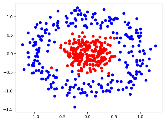
Training a model to classify points based on this dataset must be done using a neural network. This is because we need multiple perceptrons working simultaneously for this model to produce accurate results.
What is a Perceptron?
At its most basic level, a perceptron is a type of artificial neuron that involves the classification of two or more variables. Its specific use case is linear classification, where the artificial neuron aims to find a function that best describes the decision boundary between two variables. If we are then given a data value the model has never seen before, it can therefore determine which class the data point belongs to.
Neural Network Visually
You have probably seen a graph representing a neural network before. The diagram below shows the flow of values from the input end to the output end.
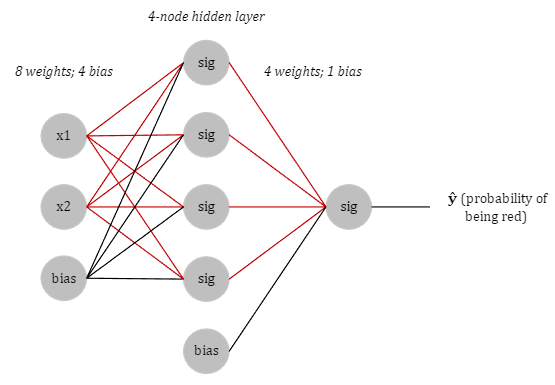
We will have 2 inputs and a bias, a 4-node hidden layer using sigmoid activation function, and a single output: the probability that a given point is red.
But how can we standardize the outputs of our model to resemble a probability? Enter sigmoid. The reason we are using sigmoid as our activation function is because our model classifies new points based on a probability, which we will call \( \hat{y} \) (pronounced “y hat”). The output of the sigmoid function lies between 0 and 1. This is perfect for us since probabilities can only exist between those values.
The reason we are using 4 sigmoid functions is quite simple. Think of it this way: what we need to do is create a sort of perimeter around the data points. That will determine a threshold of sorts, where once a value has passed in either the \( x_1 \) or \( x_2 \) direction, a value becomes red.

Neural Network Programmatically
Below is the generic template form of a neural network.
import torch
import torch.nn as nn
from torch.nn import Linear


class Model(nn.Module):

    def __init__(self, input_size, H, output_size):
        super().__init__()

        # input layer to hidden layer
        self.linear = torch.nn.Linear(input_size, H)

        # hidden layer to output layer
        self.linear2 = torch.nn.Linear(H, output_size)

    # forward pass
    def forward(self, x):
        # uses sigmoid to determine probabilities as it goes through both models
        x = torch.sigmoid(self.linear(x))
        x = torch.sigmoid(self.linear2(x))
        return x

    # make a prediction about a value x
    def predict(self, x):
    	# pred is the probability of a positive result
        pred = self.forward(x)

        return [1, pred] if pred >= .5 else [0, pred]
Training the Network
First we must convert our datasets to column matrices.
X_tensor = torch.tensor(X).float()                  # already a column matrix
Y_tensor = torch.tensor(Y).reshape(-1,1).float()    # ML needs column matrices
Now for the main part, which is training a model on our dataset. The process we must follow is:
-
Set a random seed to ensure reproducibility.
-
Call on our
Model()class to mimic the network schema. -
We use BCE as our loss algorithm, as it handles logarithms.
-
We use the
torch.optim.Adam()optimizer because it changes learning rate dynamically. -
Train model for \( x \) number of epochs so long as the model doesn’t overfit or underfit data.
# set seed for consistency of randoms
torch.manual_seed(1)

# recreate network schema
model = Model(input_size=2, H=4, output_size=1)

# training setup
epochs = 130
criterion = nn.BCELoss()
optimizer = torch.optim.Adam(model.parameters(), lr=.1)

# training model
for i in range(epochs):

    # training process
    optimizer.zero_grad()
    Yhat = model.forward(X_tensor)		# pass X data through the neural network
    loss = criterion(Yhat, Y_tensor)	# compare the predicted values with actual Y values
    loss.backward()						# find derivative
    optimizer.step()					# take the step

    # print model parameters each iteration
    print(i+1)
    print(loss)
    print(list(model.parameters()))
    print()
Visualize the Training Process
Here is a GIF that shows the visualization of the training process. It uses a contourf() plot to show the decision boundaries between the red and blue classes. Areas with lighter color represent a reduced probability that a given data point is either red or blue, though any value \( P \ge 0.5 \) is considered red.
The last step is to ask the model to classify a new point that it has never seen before. We’ll use the black point at \( (-0.5, -0.4) \) for this.
# make a prediction
print(model.predict(torch.tensor([-0.5, -0.4])))
[1, tensor([0.6090], grad_fn=<SigmoidBackward0>)]
This means that our model predicted True for the black point. Recall, that our prediction, \( \hat{y} \), represents the probability that a given point is of the red class. With this in mind, the black point is to be put in the red class, with a 60.9% probability. This value is only moderately greater than 50%, representing a moderately confident prediction. This is also apparent visually, with only a slight red coloring on the graph around the black point.
Completed Code
Here is the completed code:
import numpy as np
import matplotlib.pyplot as plt
from sklearn import datasets
import torch
import torch.nn as nn
from torch.nn import Linear

#############################
### DEFINE NEURAL NETWORK ###
#############################
class Model(nn.Module):

    def __init__(self, input_size, H, output_size):
        super().__init__()
        self.linear = torch.nn.Linear(input_size, H)
        self.linear2 = torch.nn.Linear(H, output_size)

    def forward(self, x):
        x = torch.sigmoid(self.linear(x))
        x = torch.sigmoid(self.linear2(x))
        return x

    def predict(self, x):
        pred = self.forward(x)
        return [1, pred] if pred >= .5 else [0, pred]

######################
### CREATE DATASET ###
######################
X,Y = datasets.make_circles(n_samples=500,
                            random_state=1,
                            noise=.15,		# controls the spread of points
                            factor=.25)		# controls closeness of the circles

X_tensor = torch.tensor(X).float()                  # already a column matrix
Y_tensor = torch.tensor(Y).reshape(-1,1).float()    # ML needs column matrices

######################
### MODEL TRAINING ###
######################
torch.manual_seed(1)

model = Model(input_size=2, H=4, output_size=1)

# for plotting purposes
x1 = np.arange(-1.5, 1.5, .1)
x2 = np.arange(-1.5, 1.5, .1)

rows, columns = np.meshgrid(x1, x2)

x = np.hstack([rows.ravel().reshape(-1,1), columns.ravel().reshape(-1,1)])
x_tensor = torch.tensor(x).float()

# training setup
epochs = 130
criterion = nn.BCELoss()
optimizer = torch.optim.Adam(model.parameters(), lr=.1)

# model training
for i in range(epochs):
    yhat = model.forward(x_tensor).float()
    yhat = yhat.reshape(rows.shape)

    plt.scatter(X[Y==0, 0], X[Y==0,1], color="blue")
    plt.scatter(X[Y==1, 0], X[Y==1, 1], color="red")
    plt.contourf(rows, columns, yhat.detach(), alpha=.4, cmap="RdBu_r")
    plt.scatter(-0.5, -0.4, color="black")
    plt.show()

    optimizer.zero_grad()
    Yhat = model.forward(X_tensor)
    loss = criterion(Yhat, Y_tensor)
    loss.backward()
    optimizer.step()